Partial Correlations (R,Python)

Course Overview

Red means that the page does not exist yet

Gray means that the page doesn’t yet have separation of different levels of understanding

Orange means that the page is started

In this website you can choose to expand or shrink the page to match the level of understanding you want.

If you do not expand any (green) subsections then you will only see the most superficial level of description about the statistics. If you expand the green subsections you will get details that are required to complete the tests, but perhaps not all the explanations for why the statistics work.

An example of a green subsection

If you expand the blue subsections you will also see some explanations that will give you a more complete understanding. If you are completing MSc-level statistics you would be expected to understand all the blue subsections.

An example of a blue subsection

Red subsections will go deeper than what is expected at MSc level, such as testing higher level concepts.

An example of a red subsection

As you may have heard, correlation does not equal causation. One possible reason for this is that there’s a third variable that explains an association. Let’s imagine that we are trying to understand whether life expectancy goes up over time and why. First of all, let’s check if lifeExpectancy is going up over time using the gapminder data:

R
Python

library(gapminder)
library(ggplot2)
library(tidyverse)

── Attaching core tidyverse packages ──────────────────────── tidyverse 2.0.0 ──
✔ dplyr     1.1.3     ✔ readr     2.1.4
✔ forcats   1.0.0     ✔ stringr   1.5.0
✔ lubridate 1.9.3     ✔ tibble    3.2.1
✔ purrr     1.0.2     ✔ tidyr     1.3.0
── Conflicts ────────────────────────────────────────── tidyverse_conflicts() ──
✖ dplyr::filter() masks stats::filter()
✖ dplyr::lag()    masks stats::lag()
ℹ Use the conflicted package (<http://conflicted.r-lib.org/>) to force all conflicts to become errors

gapminder %>% 
  group_by(year) %>% 
  summarise(
    lifeExp = mean(lifeExp),
    gdpPercap = mean(gdpPercap)
  ) -> gapminder_by_year

cor.test(gapminder_by_year$year, gapminder_by_year$lifeExp)


    Pearson's product-moment correlation

data:  gapminder_by_year$year and gapminder_by_year$lifeExp
t = 18.808, df = 10, p-value = 3.91e-09
alternative hypothesis: true correlation is not equal to 0
95 percent confidence interval:
 0.9498070 0.9962336
sample estimates:
     cor 
0.986158

ggplot(data = gapminder_by_year, aes(x = year, y = lifeExp)) + 
  geom_point() + 
  geom_smooth(method = lm, formula = 'y ~ x')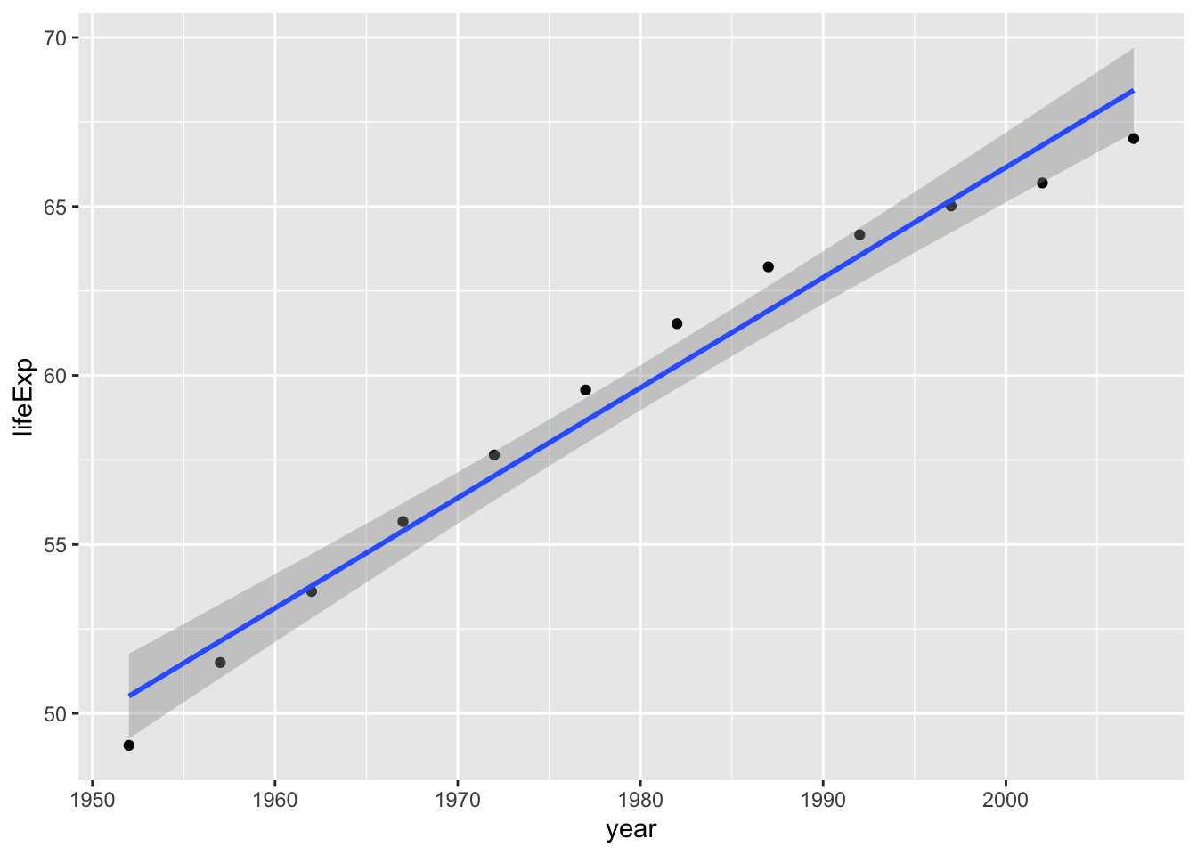

Figure 1: a scatterplot showing the association between year and life expectancy using Gapminder data.

import pandas as pd
import numpy as np
import matplotlib.pyplot as plt
import seaborn as sns
from scipy.stats import pearsonr
from gapminder import gapminder

gapminder_by_year = gapminder.groupby('year').agg({'lifeExp': 'mean', 'gdpPercap': 'mean'}).reset_index()
print(gapminder_by_year)

correlation, p_value = pearsonr(gapminder_by_year['year'], gapminder_by_year['lifeExp'])
print("Correlation coefficient:", correlation)
print("p-value:", p_value)

sns.scatterplot(data=gapminder_by_year, x='year', y='lifeExp')
sns.regplot(data=gapminder_by_year, x='year', y='lifeExp')
plt.xlabel('Year')
plt.ylabel('Life Expectancy')
plt.show()

So now that we’ve confirmed that there is a positive association between the year and life expectancy, the next question is why? What changes from year to year that could explain increased life expectancy? Let’s investigate whether gdp per capita generally goes up each year, and whether it’s associated with life expectancy. If both of these things are true, then perhaps the increase in gdp per year is an explanation of the association between year and life expectancy.

cor.test(gapminder_by_year$year, gapminder_by_year$gdpPercap)


    Pearson's product-moment correlation

data:  gapminder_by_year$year and gapminder_by_year$gdpPercap
t = 17.039, df = 10, p-value = 1.022e-08
alternative hypothesis: true correlation is not equal to 0
95 percent confidence interval:
 0.9393538 0.9954265
sample estimates:
      cor 
0.9832101

ggplot(data = gapminder_by_year, aes(x = year, y = gdpPercap)) + 
  geom_point() + 
  geom_smooth(method = lm, formula = 'y~x')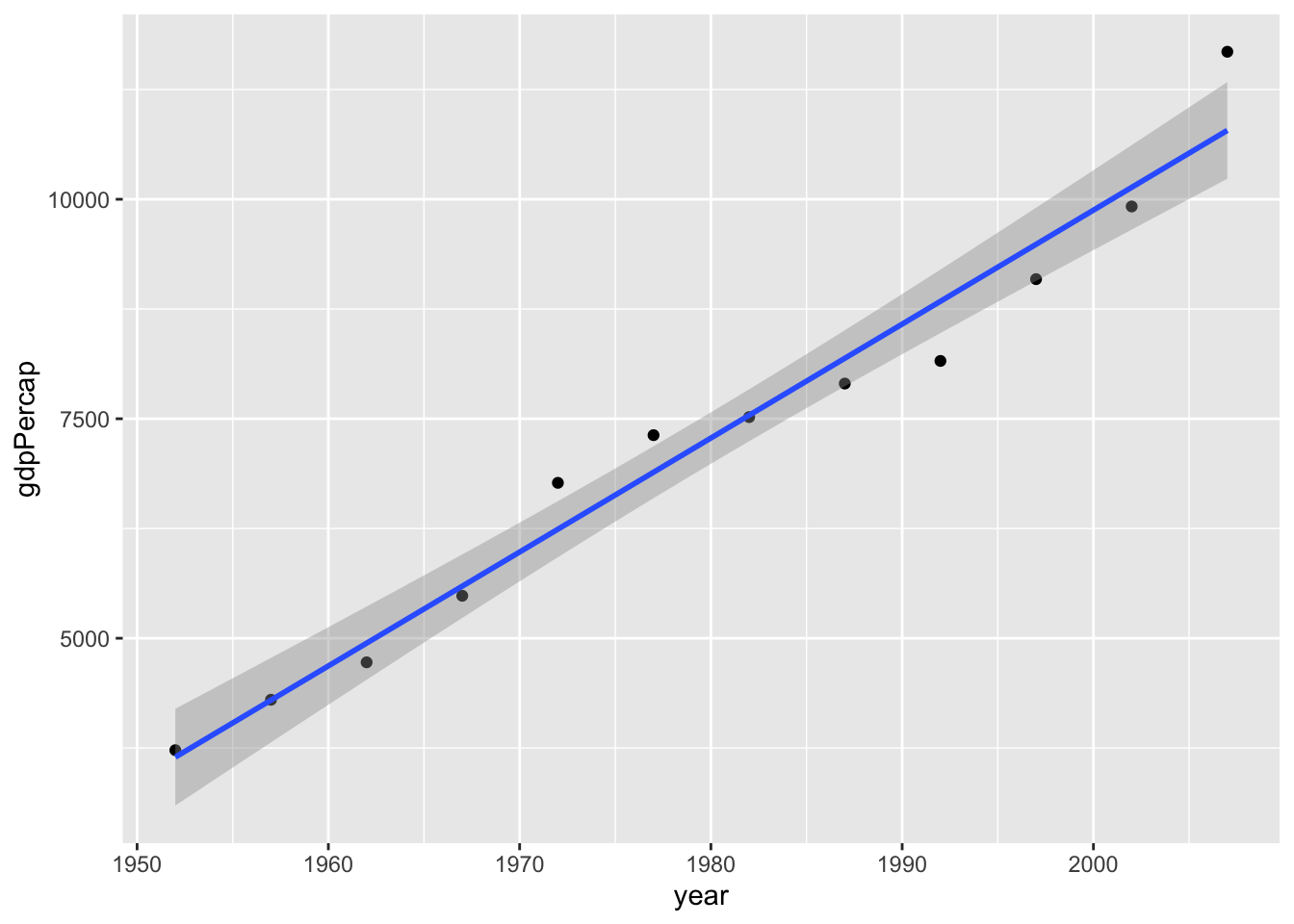

Figure 2: a scatterplot showing the association between year and GDP per Capita using Gapminder data.

correlation, p_value = pearsonr(gapminder_by_year['year'], gapminder_by_year['gdpPercap'])
print("Correlation coefficient:", correlation)
print("p-value:", p_value)

sns.scatterplot(data=gapminder_by_year, x='year', y='gdpPercap')
sns.regplot(data=gapminder_by_year, x='year', y='gdpPercap')
plt.xlabel('Year')
plt.ylabel('gdpPercap')
plt.show()

Whilst there are some outliers in earlier years, we seem to have found that gdp per capita has gone up.

Is gdp per capita and life expectancy associated?

R
Python

cor.test(gapminder_by_year$gdpPercap, gapminder_by_year$lifeExp)


    Pearson's product-moment correlation

data:  gapminder_by_year$gdpPercap and gapminder_by_year$lifeExp
t = 11.137, df = 10, p-value = 5.875e-07
alternative hypothesis: true correlation is not equal to 0
95 percent confidence interval:
 0.8663785 0.9895601
sample estimates:
      cor 
0.9619721

ggplot(data = gapminder_by_year, aes(x = gdpPercap, y = lifeExp)) + 
  geom_point() + 
  geom_smooth(method = lm, formula = 'y ~ x')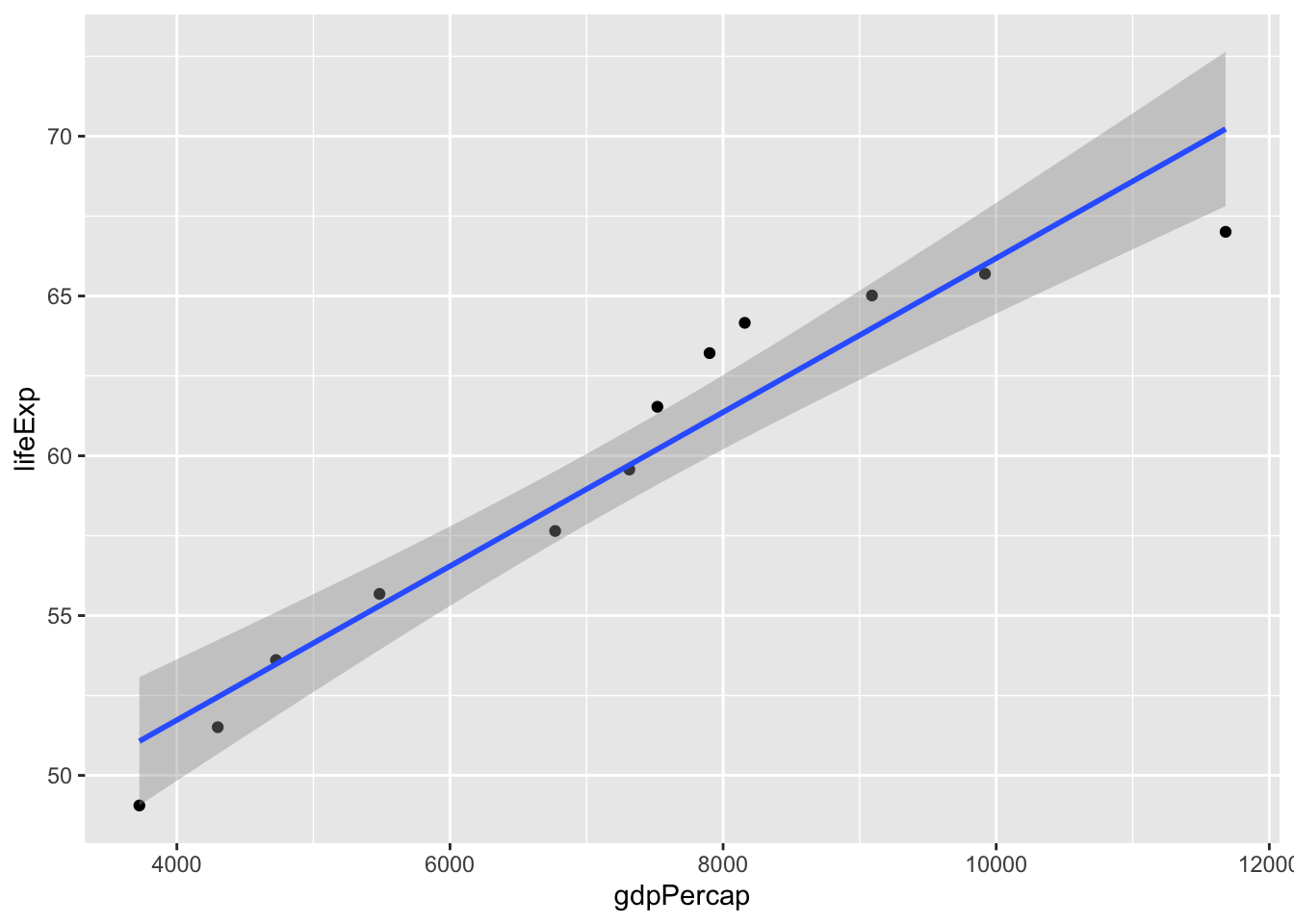

Figure 3: a scatterplot showing the association between GDP per Capita and life expectancy using Gapminder data.

# Perform correlation test between gdpPercap and lifeExp
correlation, p_value = stats.pearsonr(gapminder_by_year['gdpPercap'], gapminder_by_year['lifeExp'])

# Print the correlation coefficient and p-value
print("Correlation coefficient:", correlation)
print("p-value:", p_value)

# Create scatter plot with regression line
sns.scatterplot(data=gapminder_by_year, x='gdpPercap', y='lifeExp')
sns.regplot(data=gapminder_by_year, x='gdpPercap', y='lifeExp', scatter=False)
plt.xlabel('GDP per capita')
plt.ylabel('Life Expectancy')
plt.show()

So the above analysis suggests that all three variables are incredibly related. (you are unlikely to see such strong associations in real psychology experiments). But let’s now check in whether there’s still an association between the year and life expectancy once you control for GDP per capita. This partial correlation can be visualised as follows:

Figure 4: The association between Year and Life expectancy could be explained by GDP.

To calculate the partial correlation r value you control for the association between the two variables

\[ r_{xy*z} = \frac{r_{xy} - r_{xz} * r_{yz}}{\sqrt{(1-r^2_{xz})(1-r^2_{yz})}} = \frac{originalCorrelation - varianceExplainedByCovariate}{varianceNotExplainedByCovariate} \]

\(x\) = The Year
\(y\) = Life expectancy
\(z\) = GDP per capita
\(\sqrt{1- r^2_{xz}}\) = variance not explained by correlation between Year(\(x\)) and GDP (\(z\))
\(\sqrt{1- r^2_{yz}}\) = variance not explained by correlation between Life Expectancy (\(y\)) and GDP (\(z\))

One way to think of the formula above is that: - the top-half represents how much variance is explained by overlap between the two main variables, subtracted by the variance of each variable with the confound - the bottom-half represents how much variance there is left to explain once you’ve removed associations between each main variable and the covariate.

Let’s see what the r value is after this partial correlation:

\[ r_{xy*z} = \frac{r_{xy} - r_{xz} * r_{yz}}{\sqrt{(1-r^2_{xz})(1-r^2_{yz})}} = \frac{.986158 - .9832101 * .9619721 }{\sqrt{(1-.9832101^2)(1-.9619721^2)}} = \frac{.040354}{.04984321} = .8092841 \]

Let’s check if the manually calculated partial r-value is the same as what R gives us:

R
Python

library(ppcor)

Loading required package: MASS


Attaching package: 'MASS'

The following object is masked from 'package:dplyr':

    select

pcor(gapminder_by_year)

$estimate
               year    lifeExp  gdpPercap
year      1.0000000  0.8092844  0.7629391
lifeExp   0.8092844  1.0000000 -0.2521280
gdpPercap 0.7629391 -0.2521280  1.0000000

$p.value
                 year    lifeExp   gdpPercap
year      0.000000000 0.00254769 0.006309324
lifeExp   0.002547690 0.00000000 0.454498736
gdpPercap 0.006309324 0.45449874 0.000000000

$statistic
              year    lifeExp  gdpPercap
year      0.000000  4.1331001  3.5404830
lifeExp   4.133100  0.0000000 -0.7816358
gdpPercap 3.540483 -0.7816358  0.0000000

$n
[1] 12

$gp
[1] 1

$method
[1] "pearson"

import pingouin as pg

# Calculate partial correlation with p-values, estimates, and statistics
partial_corr1 = pg.partial_corr(data=gapminder_by_year, x="gdpPercap", y="lifeExp", covar="year", method='pearson')
partial_corr2 = pg.partial_corr(data=gapminder_by_year, x="year", y="gdpPercap", covar="lifeExp", method='pearson')
partial_corr3 = pg.partial_corr(data=gapminder_by_year, x="lifeExp", y="year", covar="gdpPercap", method='pearson')

coef1 = partial_corr1['r'].values[0]
coef2 = partial_corr2['r'].values[0]
coef3 = partial_corr3['r'].values[0]

p_value1 = partial_corr1['p-val'].values[0]
p_value2 = partial_corr2['p-val'].values[0]
p_value3 = partial_corr3['p-val'].values[0]

# Create a matrix
matrix1 = np.zeros((3, 3))

# Assign the interaction values
matrix1[0, 1] = coef3
matrix1[1, 0] = coef3
matrix1[0, 2] = coef2
matrix1[2, 0] = coef2
matrix1[1, 2] = coef1
matrix1[2, 1] = coef1

# Set the diagonal to 1
np.fill_diagonal(matrix1, 1)

# Create a DataFrame from the matrix
matrix_coef = pd.DataFrame(matrix1, columns=['year', 'lifeExp', 'gdpPercap'], index=['year', 'lifeExp', 'gdpPercap'])

# Create a matrix
matrix2 = np.zeros((3, 3))

# Assign the interaction values
matrix2[0, 1] = p_value3
matrix2[1, 0] = p_value3
matrix2[0, 2] = p_value2
matrix2[2, 0] = p_value2
matrix2[1, 2] = p_value1
matrix2[2, 1] = p_value1

# Set the diagonal to 1
np.fill_diagonal(matrix2, 1)

# Create a DataFrame from the matrix
matrix_p_val = pd.DataFrame(matrix2, columns=['year', 'lifeExp', 'gdpPercap'], index=['year', 'lifeExp', 'gdpPercap'])

# Print the resulting matrix
print(matrix_p_val)

# Print the resulting matrix
print(matrix_coef)

Yes, the pearson correlation between year and life expectancy is .8092844, so the difference of .0000003 is a rounding error from the manual calculations above. Just to confirm that this is a rounding error, here’s what you get if you complete the same steps but with the estimate part of the correlation objects instead:

R
Python

x.y.cor <- cor.test(gapminder_by_year$year, gapminder_by_year$lifeExp)
x.z.cor <- cor.test(gapminder_by_year$year, gapminder_by_year$gdpPercap)
y.z.cor <- cor.test(gapminder_by_year$gdpPercap, gapminder_by_year$lifeExp)

(x.y.cor$estimate - x.z.cor$estimate * y.z.cor$estimate)/sqrt((1-x.z.cor$estimate^2) * (1 - y.z.cor$estimate^2))

      cor 
0.8092844

import scipy.stats as stats
import numpy as np

# Calculate correlation coefficients
x_y_cor = stats.pearsonr(gapminder_by_year['year'], gapminder_by_year['lifeExp'])[0]
x_z_cor = stats.pearsonr(gapminder_by_year['year'], gapminder_by_year['gdpPercap'])[0]
y_z_cor = stats.pearsonr(gapminder_by_year['gdpPercap'], gapminder_by_year['lifeExp'])[0]

# Calculate the desired value
result = (x_y_cor - x_z_cor * y_z_cor) / np.sqrt((1 - x_z_cor**2) * (1 - y_z_cor**2))

# Print the result
print(result)

Confirming that the difference in the manual calculation is a rounding error. Note that the numbers you get from R may be rounded numbers, and so your calculations may reflect the rounding.

To conclude, as there is still an association between Year and Life Expectancy once controlling for GDP, this partial correlation is consistent with GDP not being the only explanation for why Life Expectancy goes up each year.

Question 1

What does a variable need to correlate with to be a viable candidate as a covariate?

viewof partial_correlations_1_response = Inputs.radio(['Both other variables','At least one other variable','No other variables']);
correct_partial_correlations_1 = 'Both other variables';
partial_correlations_1_result = {
  if(partial_correlations_1_response == correct_partial_correlations_1){
    return 'Correct!';
  } else {
    return 'Incorrect or incomplete.';
  };
}