Skewness (R,Python)

Course Overview

Red means that the page does not exist yet

Gray means that the page doesn’t yet have separation of different levels of understanding

Orange means that the page is started

In this website you can choose to expand or shrink the page to match the level of understanding you want.

If you do not expand any (green) subsections then you will only see the most superficial level of description about the statistics. If you expand the green subsections you will get details that are required to complete the tests, but perhaps not all the explanations for why the statistics work.

An example of a green subsection

If you expand the blue subsections you will also see some explanations that will give you a more complete understanding. If you are completing MSc-level statistics you would be expected to understand all the blue subsections.

An example of a blue subsection

Red subsections will go deeper than what is expected at MSc level, such as testing higher level concepts.

An example of a red subsection

Parametric analyses are based on the assumption that the data you are analysing is normally distributed (see below):

R
Python

library(ggplot2)
# https://stackoverflow.com/a/12429538
norm_x<-seq(-4,4,0.001)

norm_data_frame<-data.frame(x=norm_x,y=dnorm(norm_x,0,1))

p<- ggplot(
  data = norm_data_frame, 
  aes(
    x = x,
    y = y
  )
) + geom_line()

 p +
   xlim(c(-3,3)) +
   geom_col(aes(fill=x)) +
   scale_fill_gradient2(low = "red", 
                       high = "blue",
                       mid =  "white",
                       midpoint = median(norm_data_frame$x))+
   
   annotate("text", x=-2.3, y=0.01, label= "13.6%") + 
   annotate("text", x=-1.5, y=0.01, label= "34.1%") + 
   annotate("text", x=-0.6, y=0.01, label= "50%") + 
   annotate("text", x=0.5, y=0.01, label= "84.1%") + 
   annotate("text", x=1.5, y=0.01, label= "97.7%") + 
   annotate("text", x=2.25, y=0.01, label= "100%") +
   geom_vline(xintercept = -2) +
   geom_vline(xintercept = -1) +
   geom_vline(xintercept = 0) +
   geom_vline(xintercept = 1) +
   geom_vline(xintercept = 2) +
   xlab("Z-score") +
   ylab("Frequency") +
   theme(legend.position="none")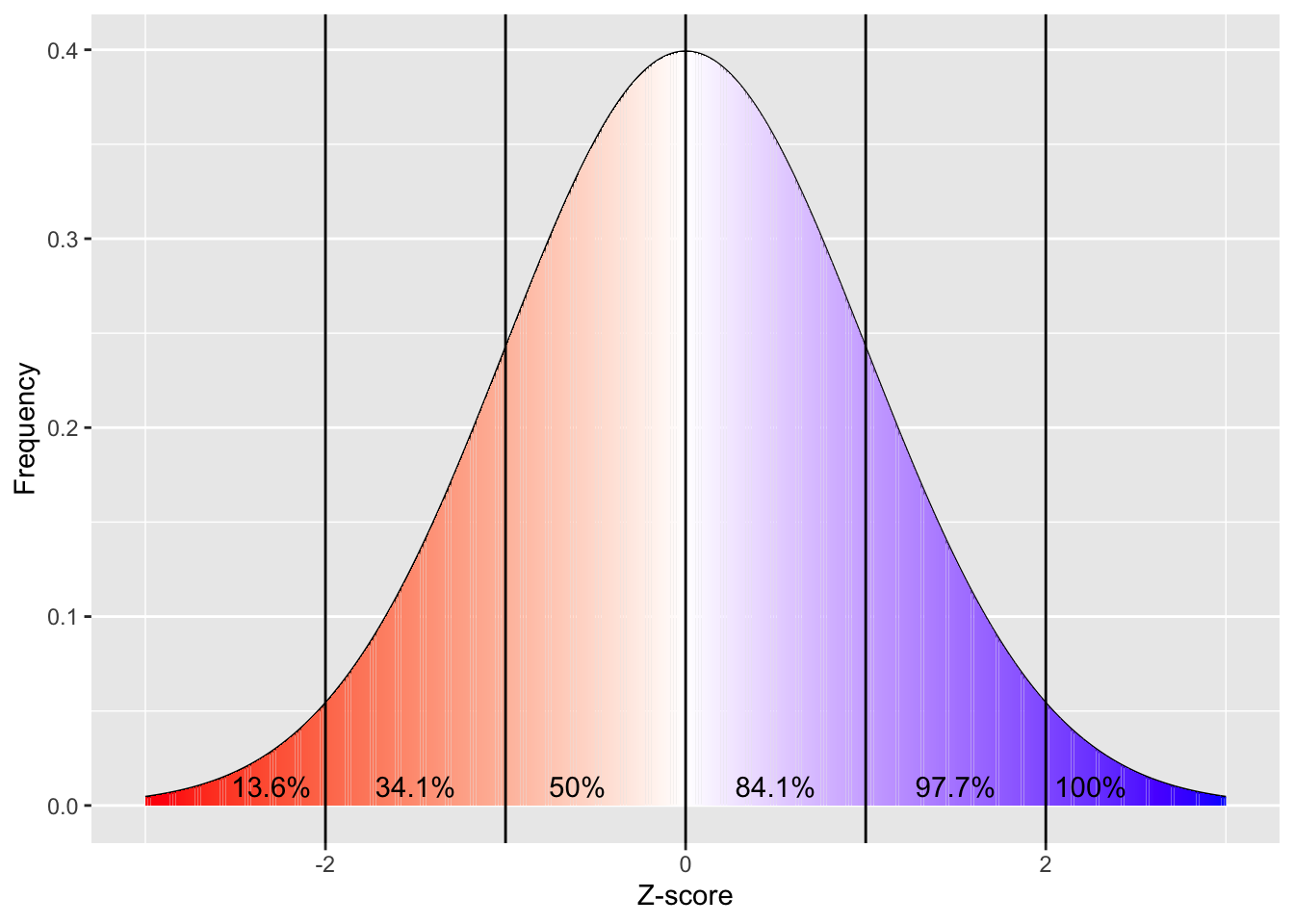

import numpy as np
import matplotlib as mpl
from scipy.stats import norm
import matplotlib.pyplot as plt

norm_x = np.arange(-4.0, 4.1, 0.1)

norm_y = norm.pdf(norm_x, loc=0, scale=1)

colourmap = mpl.cm.get_cmap('jet')

fig, ax = plt.subplots()

fig.set_figheight(7)
fig.set_figwidth(10)

ax.plot(norm_x, norm_y, color='black', alpha=1.00)
normalize = mpl.colors.Normalize(vmin=norm_y.min(), vmax=norm_y.max())
npts = 80
for i in range(npts - 1):
    plt.fill_between([norm_x[i], norm_x[i+1]],
                     [norm_y[i], norm_y[i+1]],
                     color=colourmap(normalize(norm_y[i]))
                     ,alpha=0.6)

plt.text(2.05, 0.001, '100%', fontsize = 10)
plt.text(1.2, 0.001, '97.7%', fontsize = 10)
plt.text(0.2, 0.001, '84.1%', fontsize = 10)
plt.text(-0.7, 0.001, '50%', fontsize = 10)
plt.text(-1.8, 0.001, '34.1%', fontsize = 10)
plt.text(-2.7, 0.001, '13.6%', fontsize = 10)

plt.axvline(x=-2, color='black', ls='-', lw=1)
plt.axvline(x=-1, color='black', ls='-', lw=1)
plt.axvline(x=0, color='black', ls='-', lw=1)
plt.axvline(x=1, color='black', ls='-', lw=1)
plt.axvline(x=2, color='black', ls='-', lw=1)




# add title on the x-axis
plt.xlabel("Z-score")

# add title on the y-axis
plt.ylabel("Frequency")

# show the plot
plt.show()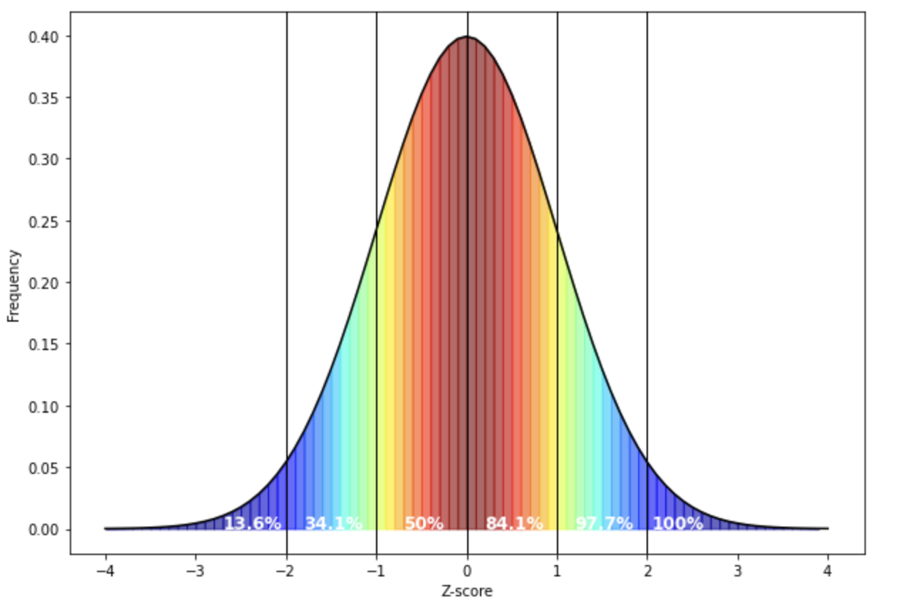

White in the above figure represents the median. Note that the mean and median overlap in a normal distribution.

If your data fits a normal distribution, then you can draw conclusions based on certain facts about this distribution, e.g. the fact that 97.7% of your population should have a score that is more negative than +2 standard deviations above the mean (because Z-scores represent standard deviations from the mean). As a result, if your data is skewed:

R
Python

library(fGarch)

skew_data_frame<-data.frame(
  x = norm_x,
  y = dsnorm(
    x = norm_x,
    mean = 0,
    sd = 1,
    xi = 2,
  )
)

ggplot(
  data = skew_data_frame, 
  aes(
    x = x,
    y = y
  )
) + 
  geom_line() + 
  geom_col(aes(fill=x)) +
  scale_fill_gradient2(low = "red", 
                       high = "blue",
                       mid =  "white",
                       midpoint = -.15)+
   theme(legend.position="none") +
  xlim(-3,3) +
  ylab("Frequency") +
  xlab("Z-score")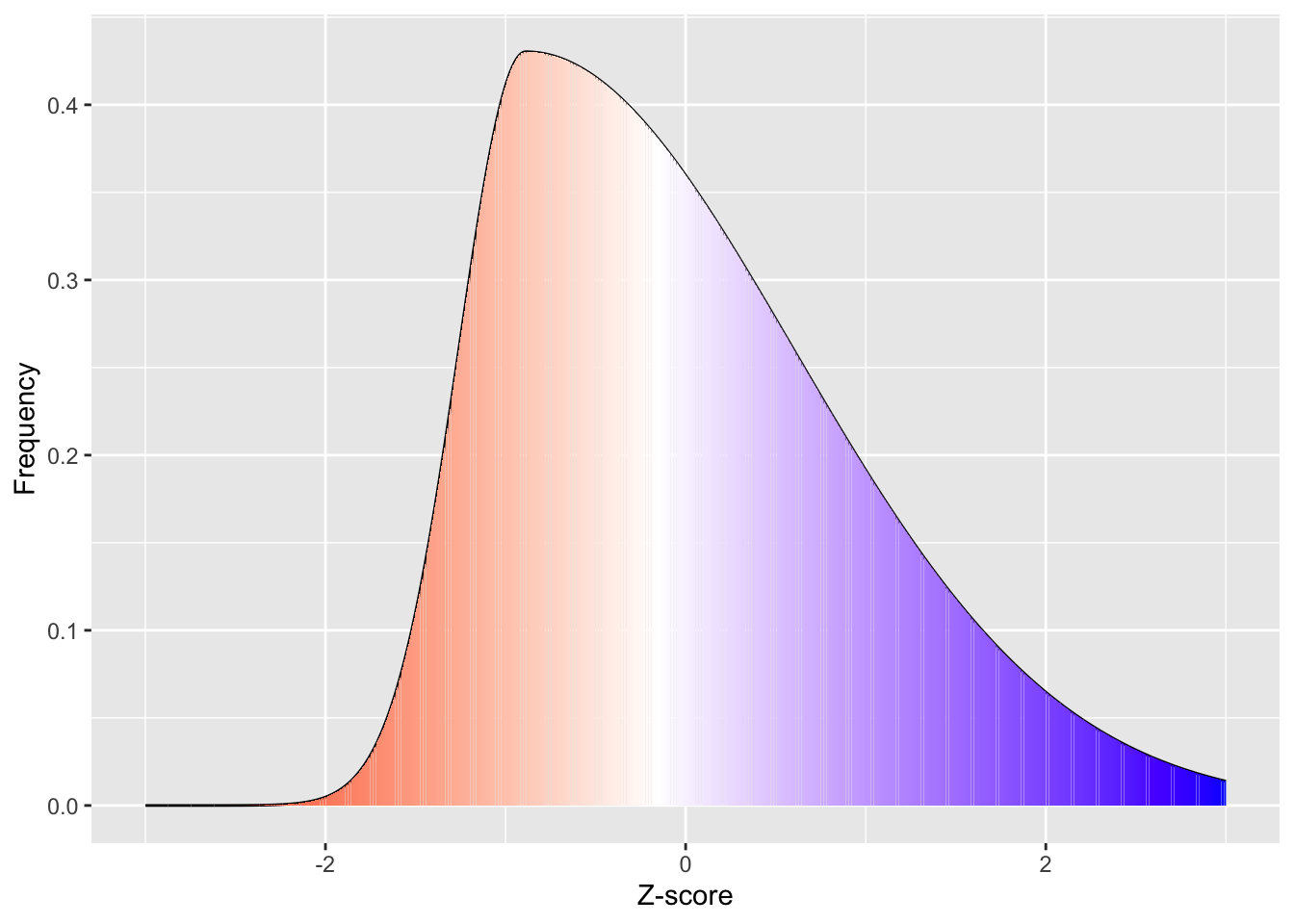

from scipy.stats import skewnorm

norm_x = np.arange(-3.0, 3.1, 0.1)

norm_y = norm.pdf(norm_x, loc=0, scale=1)
norm_y = skewnorm.pdf(norm_x, a=-2)

colourmap = mpl.cm.get_cmap('jet')

fig, ax = plt.subplots()

fig.set_figheight(7)
fig.set_figwidth(10)

ax.plot(norm_x, norm_y, color='black', alpha=1.00)
normalize = mpl.colors.Normalize(vmin=norm_y.min(), vmax=norm_y.max())
npts = 60
for i in range(npts - 1):
    plt.fill_between([norm_x[i], norm_x[i+1]],
                     [norm_y[i], norm_y[i+1]],
                     color=colourmap(normalize(norm_y[i]))
                     ,alpha=0.5)

plt.axvline(x=-0.5, color='white', ls='-', lw=1)


# add title on the x-axis
plt.xlabel("Z-score")

# add title on the y-axis
plt.ylabel("Frequency")

# show the plot
plt.show()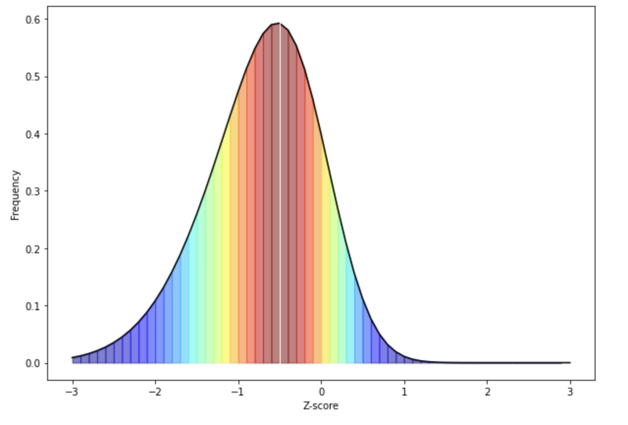

White represents the median in the figure above. As you can see from the above skewed distribution, the median is below the mean, consistent with the data being skewed. Importantly, the assumptions that we can make about what proportion of the population are 1 standard deviation above and below the mean are no longer valid, as more than half the population are below the mean in this case. This would suggest that non-parametric analyses could be more appropriate if your data is skewed.

So now that we know what skewed distributions look like, we now need to quantify how much of a problem with skewness there is.

The next section is a breakdown of the formula for those interested in it (but this is not crucial).

Optional

If we want to manually calculate skewness:

\[ \tilde{\mu_{3}} = \sum((\frac{x_i- \bar{x}{}} {\sigma} )^3) * \frac{N}{(N-1) * (N-2)} \] To do this in R you could calculate it manually. We’ll use Gapminder’s data from 2007:

R
Python

library(gapminder)

# create a new data frame that only focuses on data from 2007
gapminder_2007 <- subset(
  gapminder,   # the data set
  year == 2007     
)

hist(gapminder_2007$lifeExp)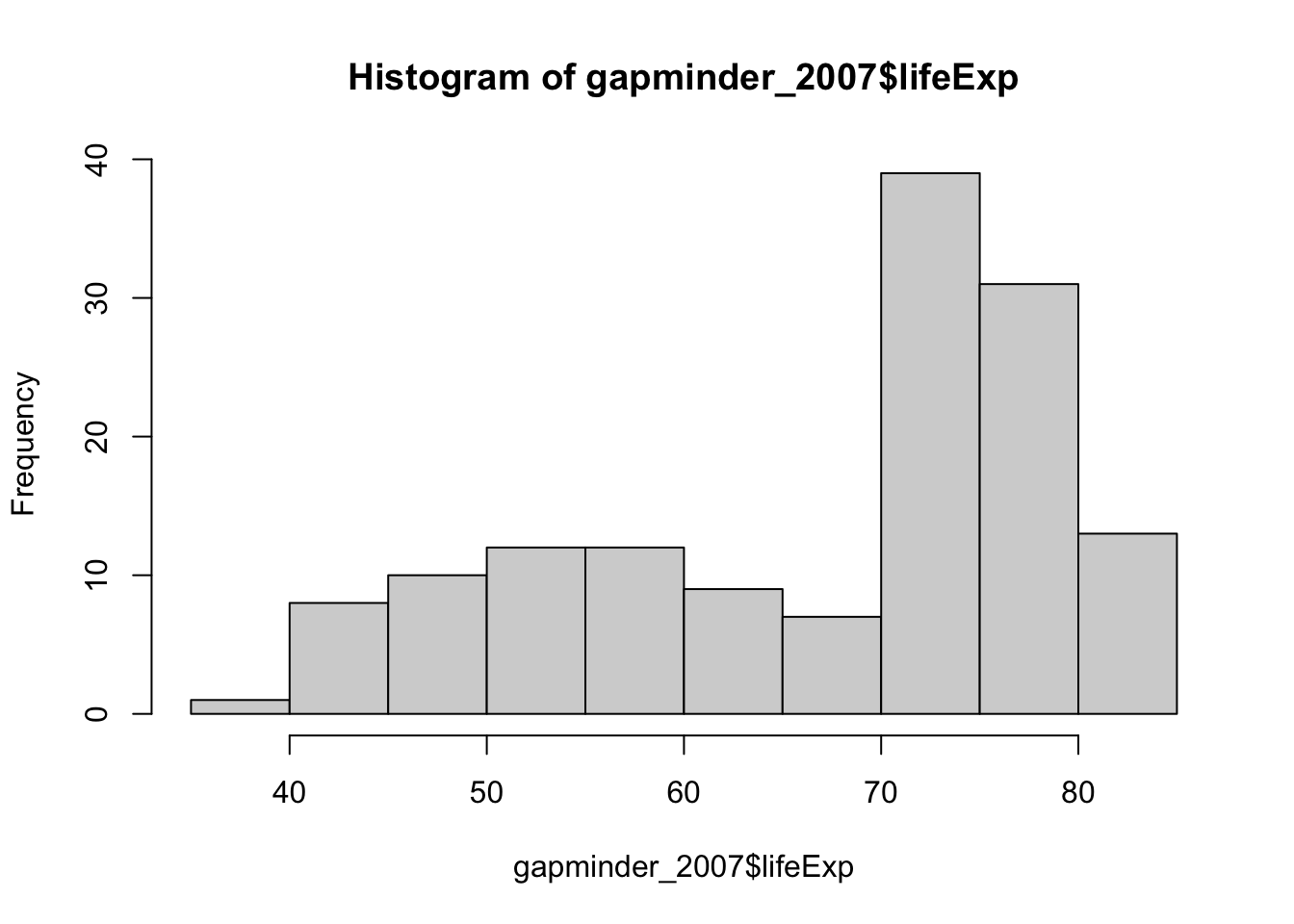

positive_skew_n = length(gapminder_2007$lifeExp)
positive_skewness = sum(((gapminder_2007$lifeExp - mean(gapminder_2007$lifeExp))/sd(gapminder_2007$lifeExp))^3) * (
  positive_skew_n / ((positive_skew_n-1) * (positive_skew_n - 2))
)
# to show the output:
positive_skewness

[1] -0.6887771

import matplotlib.pyplot as plt
import numpy as np
import math

# load the gapminder module and import the gapminder dataset
from gapminder import gapminder

# create a new data frame that only focuses on data from 2007
gapminder_2007 = gapminder.loc[gapminder['year'] == 2007]

fig, ax = plt.subplots(figsize =(7, 5))
ax.hist(gapminder_2007['lifeExp'], bins=10, color='grey',edgecolor = "black", alpha =0.8)
# add title on the x-axis
plt.xlabel("gapminder_2007['lifeExp']")

# add title on the y-axis
plt.ylabel("Frequency")

# show the plot
plt.show()

positive_skew_n = len(gapminder_2007['lifeExp'])
positive_skewness = sum(((gapminder_2007['lifeExp'] - gapminder_2007['lifeExp'].mean())/gapminder_2007['lifeExp'].std())**3) * (
  positive_skew_n / ((positive_skew_n-1) * (positive_skew_n - 2))
)

# to show the output:
positive_skewness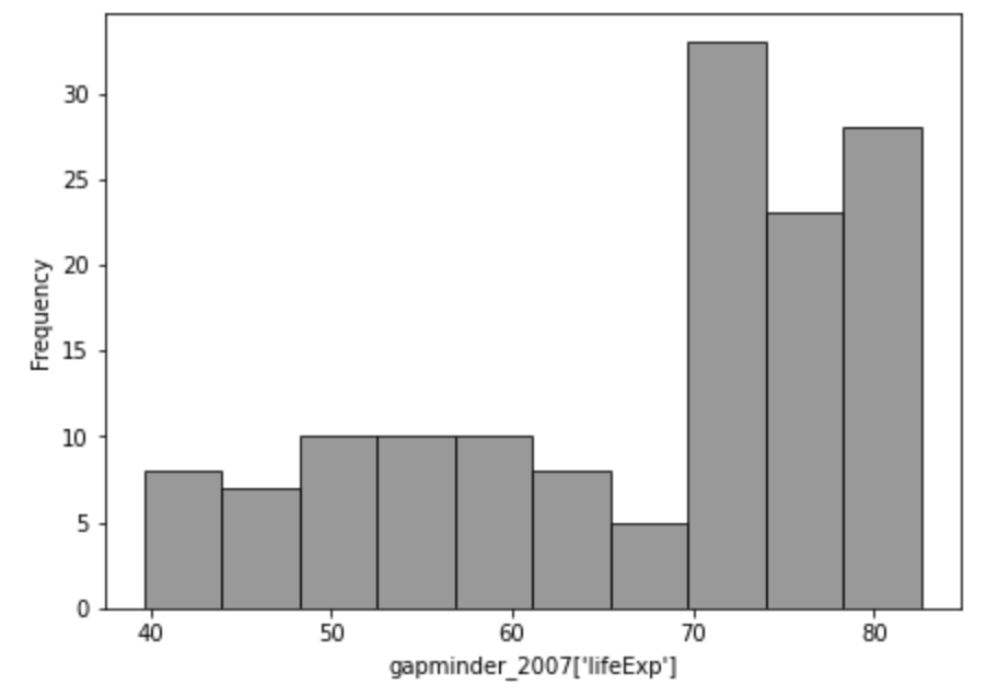

-0.68877706485775

… or just

Use code from https://stackoverflow.com/a/54369572 to give you values for skewness (this has been chosen as this gives skewness and its standard error as calculated by major software like SPSS and JASP):

R
Python

# Skewness and kurtosis and their standard errors as implement by SPSS
#
# Reference: pp 451-452 of
# http://support.spss.com/ProductsExt/SPSS/Documentation/Manuals/16.0/SPSS 16.0 Algorithms.pdf
# 
# See also: Suggestion for Using Powerful and Informative Tests of Normality,
# Ralph B. D'Agostino, Albert Belanger, Ralph B. D'Agostino, Jr.,
# The American Statistician, Vol. 44, No. 4 (Nov., 1990), pp. 316-321

spssSkewKurtosis=function(x) {
  w=length(x)
  m1=mean(x)
  m2=sum((x-m1)^2)
  m3=sum((x-m1)^3)
  m4=sum((x-m1)^4)
  s1=sd(x)
  skew=w*m3/(w-1)/(w-2)/s1^3
  sdskew=sqrt( 6*w*(w-1) / ((w-2)*(w+1)*(w+3)) )
  kurtosis=(w*(w+1)*m4 - 3*m2^2*(w-1)) / ((w-1)*(w-2)*(w-3)*s1^4)
  sdkurtosis=sqrt( 4*(w^2-1) * sdskew^2 / ((w-3)*(w+5)) )
  
  ## z-scores added by reading-psych
  zskew = skew/sdskew
  zkurtosis = kurtosis/sdkurtosis

  mat=matrix(c(skew,kurtosis, sdskew,sdkurtosis, zskew, zkurtosis), 2,
        dimnames=list(c("skew","kurtosis"), c("estimate","se","zScore")))
  return(mat)
}
spssSkewKurtosis(gapminder_2007$lifeExp)

           estimate        se    zScore
skew     -0.6887771 0.2034292 -3.385832
kurtosis -0.8298204 0.4041614 -2.053191

# Skewness and kurtosis and their standard errors as implement by SPSS
#
# Reference: pp 451-452 of
# http://support.spss.com/ProductsExt/SPSS/Documentation/Manuals/16.0/SPSS 16.0 Algorithms.pdf
# 
# See also: Suggestion for Using Powerful and Informative Tests of Normality,
# Ralph B. D'Agostino, Albert Belanger, Ralph B. D'Agostino, Jr.,
# The American Statistician, Vol. 44, No. 4 (Nov., 1990), pp. 316-321
def spssSkewKurtosis(x):
    import pandas as pd
    import math
    
    w=len(x)
    m1=x.mean()
    m2=sum((x-m1)**2)
    m3=sum((x-m1)**3)
    m4=sum((x-m1)**4)
    s1=(x).std()
    skew=w*m3/(w-1)/(w-2)/s1**3
    sdskew=math.sqrt( 6*w*(w-1) / ((w-2)*(w+1)*(w+3)) )
    kurtosis=(w*(w+1)*m4 - 3*m2**2*(w-1)) / ((w-1)*(w-2)*(w-3)*s1**4)
    sdkurtosis=math.sqrt( 4*(w**2-1) * sdskew**2 / ((w-3)*(w+5)) )
    
    ## z-scores added by reading-psych
    zskew = skew/sdskew
    zkurtosis = kurtosis/sdkurtosis
    
    mat = pd.DataFrame([[skew, sdskew, zskew],[kurtosis, sdkurtosis, zkurtosis]], columns=['estimate','se','zScore'], index=['skew','kurtosis'])
    
    return mat
  
spssSkewKurtosis(gapminder_2007["lifeExp"])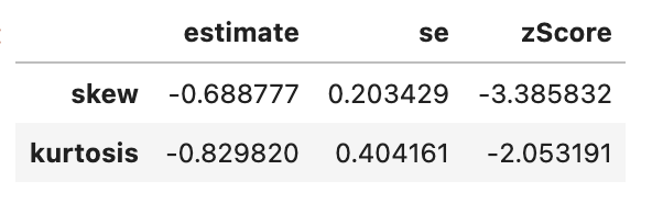

The above function generated three columns: \(estimate\) of skewness (and kurtosis, but we’ll deal with kurtosis separately, \(standard\) \(error\) (SE) and the \(skewness_z\) score. Z-scores can capture how unlikely the \(skewness\) estimate is considering what you would normally expect. In this case, when you divide skewness by standard error, you get a z-score, and if the absolute value (i.e. ignoring whether it is positive or negative) of the z-score is greater than 1.96 then it is significantly skewed. If you want to understand why 1.96 is the main number, check out the subsection on normal distributions.

One way to deal with skewed data is to transform the data.

Consolidation questions

Question 1

rand_skew_no = Math.round(Math.random() * 400)/100;

Is a skewness z-score of indicative of a significant problem of skewness?

viewof skewness_question_1_response = Inputs.radio(["Yes", "No"], {label: "", value: "A"});
this_result = { 
  var skewness_question_1_result = "awaiting response";

  if(rand_skew_no > 1.96){
    if(skewness_question_1_response == "Yes"){
      skewness_question_1_result = "Correct - Z scores above 1.96 suggest significant problems with skewness";
    } else if(skewness_question_1_response == "No") {
      skewness_question_1_result = "Not Correct - Z scores above 1.96 suggest significant problems with skewness";
    }
  } else {
    if(skewness_question_1_response == "Yes"){
      skewness_question_1_result = "Not Correct - Z scores below 1.96 **do not** suggest significant problems with skewness";
    } else if(skewness_question_1_response == "No") {
      skewness_question_1_result = "Correct  - Z scores below 1.96 **do not** suggest significant problems with skewness";
    }
  }
  return skewness_question_1_result;
}

Your answer is