Binomial Distribution (R)

Course Overview

Red means that the page does not exist yet

Gray means that the page doesn’t yet have separation of different levels of understanding

Orange means that the page is started

In this website you can choose to expand or shrink the page to match the level of understanding you want.

If you do not expand any (green) subsections then you will only see the most superficial level of description about the statistics. If you expand the green subsections you will get details that are required to complete the tests, but perhaps not all the explanations for why the statistics work.

An example of a green subsection

If you expand the blue subsections you will also see some explanations that will give you a more complete understanding. If you are completing MSc-level statistics you would be expected to understand all the blue subsections.

An example of a blue subsection

Red subsections will go deeper than what is expected at MSc level, such as testing higher level concepts.

An example of a red subsection

What is a Binomial distribution?

Imagine that you want to predict the likelihood of flipping a coin on heads or tails a certain number of times in a row. The outcome of each coin flip is binary, i.e. there is only 1 possible outcome out of 2 options. If this isn’t a biased coin, we can calculate some basic expectations about what will happen after 2 flips of the coin:

Each flip of the coin has a 50% or 0.5 chance of landing on Heads.
If we wanted to calculate the likelihood of 2 flips of heads, there’s a 0.5 chance we get the first heads flip, and then another 0.5 chance we’ll get the second head flip. To summarise this, we can multiply both 0.5 chances together to get .025.
To summarise the likelihood of all combinations we could make the following table:

First flip and likelihood	Second flip and likelihood	Overall likelihood
Heads (.5)	Heads (.5)	0.5 * 0.5 = .25
Heads (.5)	Tails (.5)	0.5 * 0.5 = .25
Tails (.5)	Heads (.5)	0.5 * 0.5 = .25
Tails (.5)	Tails (.5)	0.5 * 0.5 = .25
	Likelihood of one of the above happening	.25 + .25 + .25 + .25 = 1

library(ggplot2)
d=data.frame(
  x1=c(0,  .5,0, .5), 
  x2=c(0.5,1 ,.5,1), 
  y1=c(0,  .5,.5,0), 
  y2=c(0.5,1 ,1 ,.5), 
 # t=c('Both heads','Both tails','Mixed','Mixed'), 
  r=c('Both heads','Both tails','Mixed','Mixed'))
ggplot() + 
scale_x_continuous(name="Flip 1") + 
scale_y_continuous(name="Flip 2") +
geom_rect(data=d, mapping=aes(xmin=x1, xmax=x2, ymin=y1, ymax=y2, fill=r), color="black", alpha=0.5) +
geom_text(data=d, aes(x=x1+(x2-x1)/2, y=y1+(y2-y1)/2, label=r), size=4)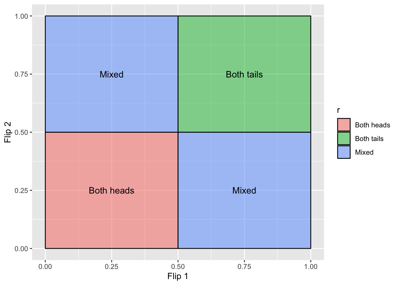

Figure 1: a summary of the likelihood of all outcomes, with the propotion of area covered by an outcome reflecting its likelihood. For example, the likelihood of flipping coins heads is .5 * .5 reflecting a .25 (or 25%) chance of flipping heads twice.

Out of these 4 combinations, the likelihood of each of them in their precise order is exactly .25 (or a 25% chance). However, we often don’t care about order, so the odds of getting 1 head and 1 tail flip would be .25 + .25 = 50% chance. This allows us to create a very simple binomial distribution of head flips:

library(ggplot2)

coin_flips <- data.frame(
  first  = c("heads","heads","tails","tails"),
  second = c("heads","tails","heads","tails"),
  heads  = c(2,1,1,0)
)

ggplot(coin_flips, aes(heads)) + geom_histogram(bins = 3)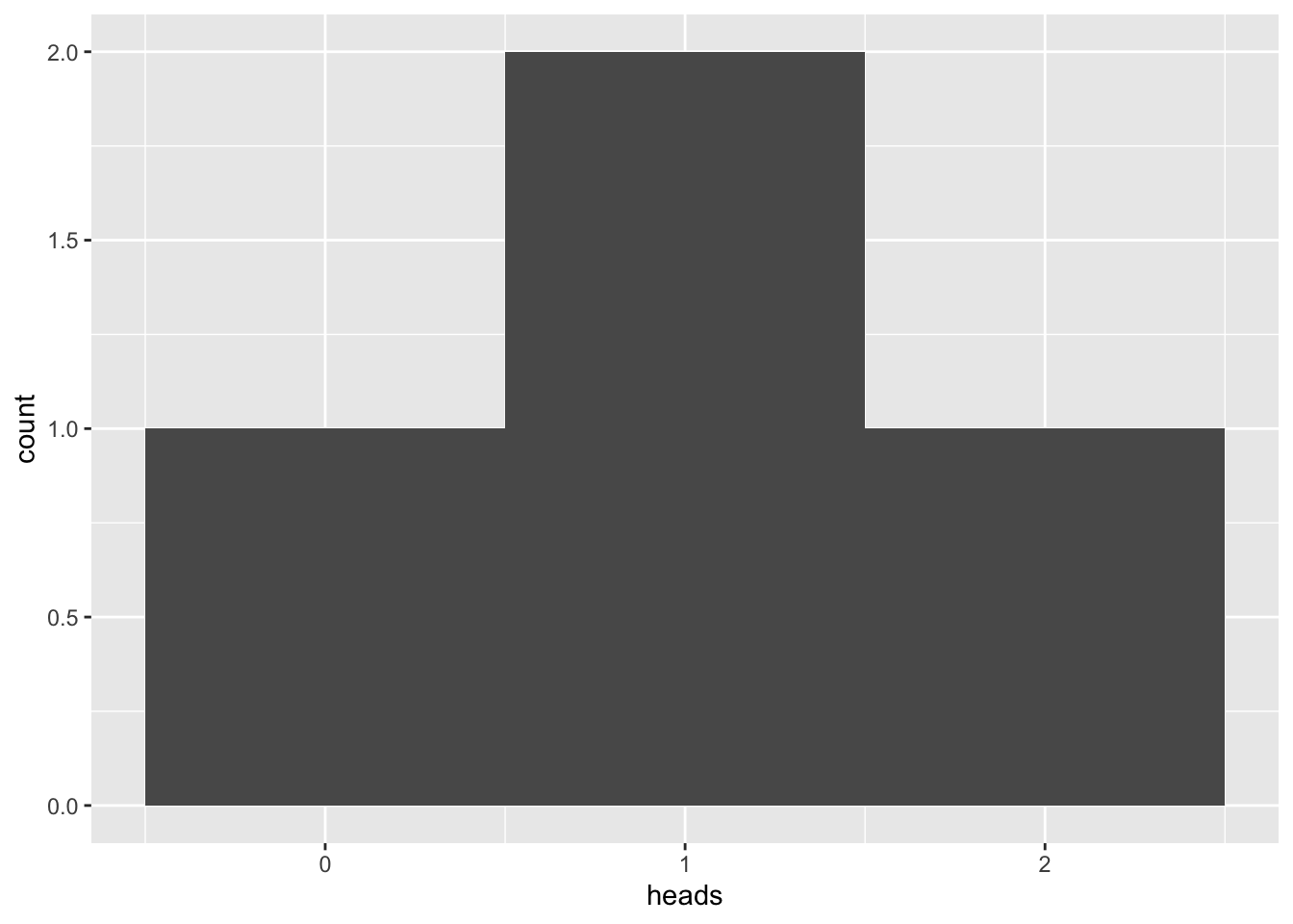

Figure 2: a binomial distribution reflecting how frequently you should expect each number of head flips.

We can calculate the likelihood of how many heads you will flip using the above distribution. Let’s say that you wanted to know the likelihood of getting at least 1 flip of heads:

ggplot(coin_flips, aes(heads, fill = heads >= 1)) + geom_histogram(bins = 3)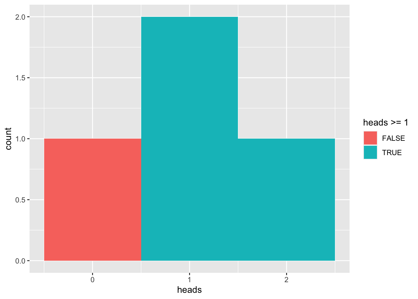

Figure 3: a binomial distribution reflecting how frequently you should expect to flip heads at least once.

You can calculate the area under this distribution this is true for, and divide it by the total area of the distribution:

sum(coin_flips$heads >= 1) / length(coin_flips$heads)

[1] 0.75

This suggests you have a 75% chance of flipping heads at least once. Looking at the table above will confirm that there is ony 1 out of 4 combinations in which you never flip heads, also supporting the fact that you will flip heads at least once the other 3 out of 4 times (i.e. 75% of the time).

What if the odds of each option are not equal to each other (e.g. you have a biased coin)

Let’s now imagine that we have a coin that will flip heads 75% of the time, and tails 25% of the time. It’s a bit more complicated to draw a distribution that captures this as the likelihood of either side is no longer equal.

biased_coin_flips <- data.frame(
  first_flip = c("heads","heads","tails","tails"),
  first_likelihood = c(.75,.75,.25,.25),
  second_flip = c("heads","tails","heads","tails"),
  second_likelihood = c(.75,.25,.75,.25),
  heads = c(2,1,1,0)
)
biased_coin_flips$outcome_likelihood = biased_coin_flips$first_likelihood * 
  biased_coin_flips$second_likelihood
# Checking if all outcomes captured (should get 1) and no overlapping outcomes (should not get more than 1). See the page on *probabilities* for more information
sum(biased_coin_flips$outcome_likelihood)

[1] 1

knitr::kable(biased_coin_flips)

first_flip	first_likelihood	second_flip	second_likelihood	heads	outcome_likelihood
heads	0.75	heads	0.75	2	0.5625
heads	0.75	tails	0.25	1	0.1875
tails	0.25	heads	0.75	1	0.1875
tails	0.25	tails	0.25	0	0.0625

If we want a histogram, we can get a sum of the outcome_likelihood for each number of heads (thus ignoring the order):

biased_heads <- data.frame(
  heads = c(0,1,2),
  freq  = c(
    sum(biased_coin_flips$outcome_likelihood[biased_coin_flips$heads == 0]),
    sum(biased_coin_flips$outcome_likelihood[biased_coin_flips$heads == 1]),
    sum(biased_coin_flips$outcome_likelihood[biased_coin_flips$heads == 2])
  )
)
ggplot(biased_heads, aes(x=heads,y=freq)) +
  geom_col() + 
  xlab("Number of head flips") +
  ylab("Frequency")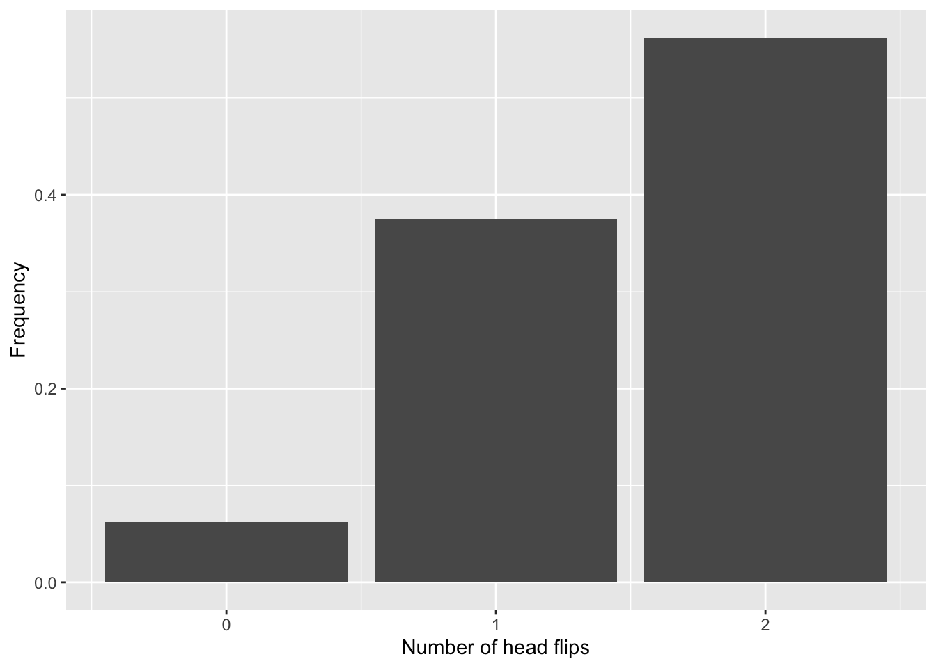

Figure 4: a binomial distribution reflecting how frequently you should expect to flip heads with a coin that has a .75 bias for heads.

How likely am I to get at least 1 head flip with this biased coin?

sum(biased_heads$freq[biased_heads$heads >= 1])

[1] 0.9375

Which can be visualised as:

ggplot(biased_heads, aes(x=heads,y=freq, fill = heads >= 1)) +
  geom_col() + 
  xlab("Number of head flips") +
  ylab("Frequency")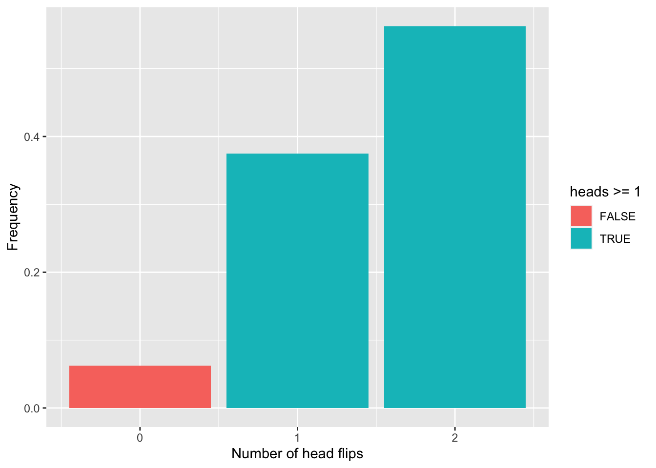

Figure 5: a binomial distribution reflecting how likely it you will flip head at least once when the coin has a .75 bias for heads.

Bivariate distributions

Note that the above distributions we’ve calculated, and thus the p-values associated with certain outcomes (or greater or lesser), use the same principles for other distributions such as t-distributions.

Question 1

Do binomial distributions only work if there is an equal likelihood of either outcome?

viewof binomial_1_response = Inputs.radio(['Yes','No']);
correct_binomial_1 = 'No';
binomial_1_result = {
  if(binomial_1_response == correct_binomial_1){
    return 'Correct!';
  } else {
    return 'Incorrect or incomplete.';
  };
}

Question 2

What is the likelihood of flipping 2 heads in a row if your coin is .6 biased towards heads

viewof binomial_2_response = Inputs.number();
correct_binomial_2 = '.36';
binomial_2_result = {
  if(binomial_2_response == correct_binomial_2){
    return 'Correct!';
  } else {
    return 'Incorrect or incomplete.';
  };
}